Machine
learning is a subfield of Artificial Intelligence and deals with the development
of techniques which allows computers to “learn” from previously seen datasets.
Machine learning overlaps extensively with mathematical statistics, but differs
in that it deals with the computational complexities of the algorithms.
Machine learning
itself can be divided into many subfields, whereas the field we will work with
is the one of supervised learning where we will start with a data set with
labeled data points. Each data point is a vector

and each data
point has a label
 .
.
Given a set
of data points and the corresponding labels we want be able to train a computer
program to classify new (so far unseen) data points by assigning a correct
class label to each data point. The ratio of correctly classified data points
is called the accuracy of the system.
Regression
analysis is a field of mathematical statistic that is well explored and has
been used for many years. Given a set of observations, one can use regression
analysis to find a model that best fits the observation data.
The most
common form of regression models is the ordinary linear regression which is
able to fit a straight line through a set of data points. It is assumed that
the data point’s values are coming from a normally distributed random variable
with a mean that can be written as a linear function of the predictors and with
a variance that is unknown but constant.
We can write
this equation as

where a
is a constant, sometimes also denoted as b0,  is a vector of the
same size as our input variable x and where the error term
is a vector of the
same size as our input variable x and where the error term
 .
.
Figure 2
shows a response with mean

which follows
a normal distribution with constant variance 1.
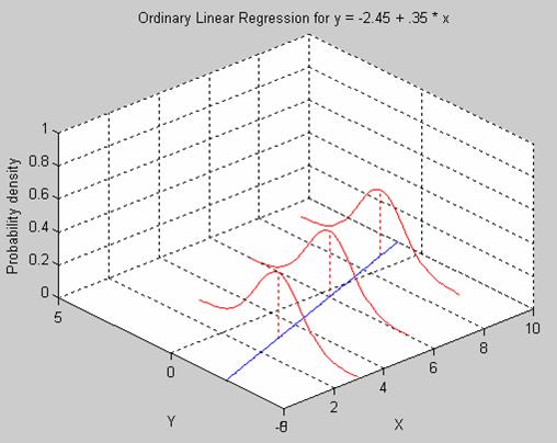
Figure 2 Ordinary Linear Regression
Ordinary Linear Regression for y = -2.45
+ 0.35 * x. The error term has mean 0 and a constant variance.
The general form
of regression, called generalized linear regression, assumes that the data
points are coming from a distribution that has a mean that comes from a
monotonic nonlinear transformation of a linear function of the predictors. If
we can call this transformation g, the equation can be written as

where a
is a constant, sometimes also denoted as b0, is a vector of the
same size as our input variable x and where the error term is  .
.
The inverse of
g is called the link function. With generalized linear regression we no longer
require the data points to have a normal random distribution, but we can have
any distribution.
Figure 3
shows a response with mean

which follows
a Poisson distribution.
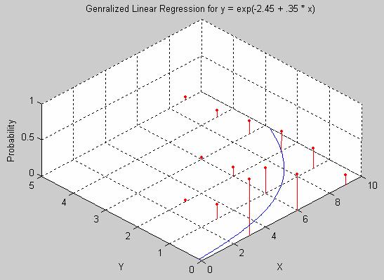
Figure 3 Generalized Linear Regression
Generalized Linear Regression for a
signal coming from a Poisson distribution with mean y = exp(-2.45 + 0.35 * x).
Although the
linear regression model is simple and used frequently it’s not adequate for
some purposes. For example, imagine the response variable y to be a probability
that takes on values between 0 and 1.
A linear model has no bounds on what values the response
variable can take, and hence y can take on arbitrary large or small values.
However, it is desirable to bound the response to values between 0 and 1. For
this we would need something more powerful than linear regression.
Another
problem with the linear regression model is the assumption that the response y
has a constant variance. This can not be the case if y follows for example a
binomial distribution (y ~ Bin(p,n)). If y also is normalized so that it takes
values between 0 and 1, hence y = Bin(p,n)/n, then the variance would then be
Var(y) = p*(1-p), which takes on values between 0 and 0.25. To then make an
assumption that y would have a constant variance is not feasible.
In situations
like this, when our response variable follows a binomial distribution, we need
to use general linear regression. A special case of general linear regression
is logistic regression, which assumes that the response variable follows the
logit-function shown in Figure 4.
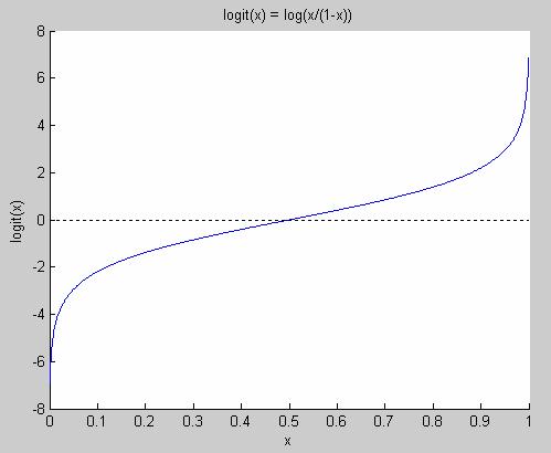
Figure 4 The logit function
Note that it’s only defined for values
between 0 and 1. The logit function goes from minus infinity to plus infinity.
The logit function has the nice property that logit(p) = -logit(1-p) and its
inverse is defined for values from minus infinity to plus infinity, and it only
takes on values between 0 and 1.
However, to
get a better understanding for what the logit-function is we will now introduce
the notation of odds. The odds of an
event that occurs with probability P is defined as
odds = P /
(1-P).
Figure 5
shows how the odds-function looks like. As we can see, the odds for an event is
not bounded and goes from 0 to infinity when the probability for that event
goes from 0 to 1.
However, it’s
not always very intuitive to think about odds. Even worse, odds are quite
unappealing to work with due to its asymmetry. When we work with probability we
have that if the probability for yes
is p, then the probability for no is
1-p. However, for odds, there exists no such nice relationship.
To take an
example: If a Boolean variable is true with probability 0.9 and false with
probability 0.1, we have that the odds for the variable to be true is 0.9/0.1 =
9 while the odds for being false is 0.1/0.9 = 1/9 = 0.1111... . This is a quite
unappealing relationship. However, if we take the logarithm of the odds, when
we would have log(9) for true and log(1/9) = -log(9) for false.
Hence, we
have a very nice symmetry for log(odds(p)). This function is called the
logit-function.
logit(p) = log(odds(p)) = log(p/(1-p))
As we can
see, it is true in general that logit(1-p)=-logit(p).
logit(1-p) = log((1-p)/p) = - log(p/(1-p))
= -logit(p)
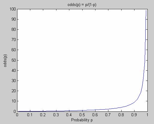
Figure 5 The odds function
The odds function maps probabilities
(between 0 and 1) to values between 0 and infinity.
The logit-function
has all the properties we wanted but did not have when we previously tried to
use linear regression for a problem where the response variable followed a
binomial distribution. If we instead use the logit-function we will have p
bounded to values between 0 and 1 and we will still have a linear expression
for our input variable x
logit(p) = a
+ * x.
If we would
like to rewrite this expression to get a function for the probability p it
would look like

In practice,
one usually simplifies notation somewhat by only having one parameter instead of both  and .
and .
If our
original problem is formulated such as

We rewrite
this as

If we now
call ’ = [] T and x’ = [1 x] then we can formulate the exact
same problem but with only “one” model parameter ’
 .
.
Note that
this is nothing but a change of notation. We still have two parameters to
determine, but we have simplified our notation so that we now only need to
estimate ’.
From now on,
we will denote ’ as and x’ as x and our
problem statement will hence be to obtain the model parameter when

If we have
made n observations with responses yi and predictors xi
we can define

 .
.
The system we
want to solve to find the parameter is then written as
 .
.
The minimum
square error solution to this system is found as follows

 .
.
We just need
to evaluate the expression (XT * X)-1 * X T *
Y and we have found the that minimizes the sum
of squares residuals. However, in practice there might be computational
difficulties with evaluating this expression, as we will see further on.
As we have
seen we can obtain by simply evaluating
.
However, if
some prediction variables are (almost) linearly dependent, then XT *
X is (almost) singular and hence he variance of is very large. So to
avoid having XT * X singular we add a small constant value to the
diagonal of the matrix

where I =
unity matrix, and λ = small constant.
By doing this
we avoid the numerical problems we will get when trying to invert an (almost)
singular matrix. But we are paying a price for doing this. By doing this we
have biased the prediction and hence we are solving the solution to a slightly
different problem. As long as the error due to the bias is smaller than the
error we would have got from having a (nearly) singular XT * X we
will end up getting a smaller mean square error and hence ridge regression is
desirable.
We can also
see ridge regression as a minimization problem where we try to find a according to

 .
.
Which we
(through Lagrange multiplier) can rewrite to an unconstraint minimization
problem

where λ
is inversely proportional to s.
This can be
compared to the classic regression where we are minimizing
.
Now the
problem is just to find a good λ (or s) so that the variance gets small,
but at the same time we should make sure the bias error doesn’t get to big
either. To find a good λ (or s) we can use heuristics, graphics or cross
validation. However, this can be computationally expensive, so in practice one
might prefer to just choose a small constant λ and then normalize the
input data so that

and
 .
.
Or in other
words, we make sure x is centered and normalized.
Ridge
regression has the advantage of preferring smaller coefficient values for and hence we end up
with a less complex model. This is desirable, due too Occam’s razor which says
that it is preferable to pick the simpler model out of two models that are
equally good but where one is simpler than the other, since the simpler model
is more likely to be correct and also hold for new unseen data.
Another way
to get an intuition for why we prefer small coefficient values is in the case
when we have correlated attributes. Imagine two attributes that are strongly
correlated and when either one of them takes the value 1, the other one does
the same with high likelihood and vice verse. It would now be possible that the
coefficients for these two attributes to take identical extremely large values
but with different signs since they both “cancel out” each other. This is of
course undesirable in the situations when the attributes take different values
and X * takes on ridiculously
large values.
Ridge
regression has proved itself to be superior to many alternative methods when it
has been used to avoid numerical difficulties when solving linear equation
systems for building logistic regression classifiers ([1], [2], [13]).
Ridge
regression was first used in the context of least square regression in [15] and
later on used in the context of logistic regression in [16].
As we have
seen we need to evaluate this expression in classic logistic regression
This
expression came from the linear equation system
.
Indirectly we
assumed that all observations where equally important and hence had the same
weight, since we tried to minimize the sum of squared residuals.
However, when
we do weighted logistic regression we will weight the importance of our
observations so that different observations have different weights associated
to them. We will have a weight matrix W that is a diagonal matrix with the
weight of observation i at location Wii.
Now, instead
of evaluating
we will
evaluate

where

and μi
is our estimate for p, which we previously saw could be written as
 .
.
The weights Wii
are nothing but the standard deviation of our own prediction. In general, if

then

and since we
have a Bernoulli trial we have n = 1 so the variance becomes
 .
.
The term yi
- μi is our prediction error and the variance Wii
“scales” it so that a low variance will have a larger impact on U than a high
variance data point. Or in other words, the importance of correctly classifying
data points with a low variance increases while the importance of correctly
classifying data points with a high variance decreases.
We have now
seen the theory behind the equation that we now need to solve. With notation as
before we now want to solve
 .
.
However, so
far we have not discussed the computational difficulties with doing this. One
of the major differences between classical statistics and machine learning is
that the later one deals with the computational difficulties one is facing when
one is trying to solve the equations obtained from the field of classical
statistics.
When one
needs to evaluate an expression such as the one we have for , it is very common to write down the problem as a linear
equation system that needs to be solved, to avoid having to calculate the
inverse of a large matrix.
Hence, the
problem can be rewritten as

where

 .
.
Let us now
take a closer look at the problem we are facing.
What we want
to achieve is to build a classifier that will classify very large data sets.
Our input data is X and (indirectly) U. To get an idea of what size our
matrices have, imagine our application having 100,000 classes and 100,000
attributes, also imagine us having in average 10 training data points per
class. The size of the A matrix would then be 100,000 x 100,000 and the size of the b vector would
be 100,000 x 1. The X matrix would be of size 1’000’000 x 100,000. Luckily for
us, our data will be sparse, and hence only a small fraction of the elements
will have non-zero values. Using this knowledge, we can choose an equation
solver that is efficient given this assumption.
In general
when one needs to solve a linear equation system such as
one needs to choose
a solver method appropriate to the properties of the problem. This basically
means that one needs to investigate what properties are satisfied for A and
from that choose one of the many available solver methods that are available.
If one needs an iterative solver, which does not give an exact solution but is
computationally efficient and in many case the only practical alternative, [3]
offers an extensive list of solvers that can be used.
For our
application we are going to use the conjugate gradient method, which is a very
efficient method for solving linear equation systems when A is a symmetric
positive definite matrix, since we only need to store a limited number of
vectors in memory.
When we solve
a linear system with iterative CG we will use the fact that the solution to the
problem A * = b, for symmetric
positive definite matrices A, is identical to the solution for the minimization
problem
 .
.
The complete algorithm
for solving using the CG algorithm
is found in Figure 6.

Figure 6 The conjugate gradient method
The conjugate gradient method can
efficiently solve the equation system
A * = b, for symmetric
positive definite sparse matrices A.
With perfect
arithmetic, we will be able to find the correct solution x in the CG algorithm
above in m steps, if A is of size m. However, since we will solve the system A
* = b iteratively, and
our A and b will change after each iteration, we don’t iterate the CG algorithm
until we have an exact solution for . We stop when is “close enough” to
the correct solution and then we recalculate A and b, using the recently
calculated value, and once again
run the CG algorithm to obtain an even better value. So although the
CG algorithm requires m steps to find the exact solution, we will terminate the
algorithm in advance and hence get a significant speed up.
How fast we
get to a solution that is good depends on the eigenvalues of the matrix A. We
earlier stated that m iterations are required to find the exact solution, but to
be more precise the number of iterations required is also bounded by the number
of distinct eigenvalues of matrix A. However, in most practical situations with
large matrices we will just iterate until the residual is small enough. Usually
we will get a solution that is reasonable good within 20-40 iterations.
Note that one
might choose many different termination criteria for when we want to stop the
CG algorithm. For example:
- Termination when we have iterated too
many times.
- Termination when residual is small
enough
 .
.
- Termination when the relative
difference of the deviance is small enough
 .
.
The deviance
for our logistic regression system is

where as
previously
.
For an
extensive investigation of how different termination criteria are affecting the
resulting classifier accuracy, see [9].
For the
reader interested in more details about the conjugate gradient method and
possible extensions to it, the authors would like to recommend [3], [7] and
[8].
Many papers
have been investigating how one can build large scale logistic classifiers with
different linear equations solvers ([1], [4], [5], [6]). We will be using the
conjugate gradient method for this task. This has previously been reported to
be a successful method for building large scale logistic classifiers in terms
of nr of attributes and in nr of data points ([1]). However, due to the fact
that the high computational complexity of calculating it is infeasible to
build very large logistic regression classifiers if we don’t have an algorithm
for building the classifier in a distributed environment using the power of a
large number of machines.
The main
contribution of this research will be to develop an efficient algorithm for
building a very large scale logistic regression classifier using a distributed
system.
We have now
gone through all theory we need to be able to build a large scale logistic
regression classifier. To obtain we will now be using
the iteratively reweighted least-squares method, also known as the IRLS method
in Figure 10.
A complete
algorithm for getting is shown in Figure 7.

Figure 7 Algorithm for Obtaining (IRLS)
The Iteratively Reweighted
Least-Squares method algorithm.
Note that
this will give us for one class only. We
need to run this algorithm once for each class that we have so that we have one
for each class. If we for
example have 100,000 classes, the algorithm would need to run 100,000 times
with different yi values each time. To run this code with a data set
with around one million data points that have in the order of 100,000
attributes could take in the order of 1 minute to finish, so to be able to
scale up our classifier we need an algorithm that can efficiently run this
piece of code on distributed client machines.
The way we
will do classification with our system when we have all values is to create a
matrix that we call the “weight matrix” (denoted W).
Say we have a
data point x and we want to know which of the n classes it should belong to.
We have
previously seen that the probability that data point x belongs to the class
corresponding to is
 .
.
Hence, the
larger value we have for * x, the stronger is
our belief that the data point x belongs to the class corresponding to . So to do classification, we only need to see which gives the highest
value and chose that class as our best guess.
 .
.
To do ranking,
we do basically the same thing as for classification
 .
.
Hence, the score for
class i will be i * x, and we rank the classes so that the class
with the highest score is ranked highest.
LIST OF ABBREVIATIONS
LR Logistic Regression
NB Naïve Bayesian
CG Conjugate Gradient
IRLS Iteratively Reweighted
Least-Squares
References
·
[1] P. Komarek and A. Moore, Making Logistic Regression A Core Data
Mining Tool: A Practical Investigation of Accuracy, Speed, and Simplicity.
ICDM 2005.
·
[2] P. Komarek and A. Moore. Fast Robust Logistic Regression for Large
Sparse Datasets with Binary Outputs. In Artificial Intelligence and
Statistics, 2003.
·
[3] R
Barrett, M Berry, T F. Chan, J Demmel, J M. Donato, J Dongarra, V Eijkhout, R
Pozo, C Romine and H Van der Vorst. Templates
for the Solution of Linear Systems: Building Blocks for Iterative Methods.
Netlib Repository.
·
[4] Christopher J. Paciorek and Louise Ryan, Computational techniques for spatial
logistic regression with large datasets. October 2005.
·
[5] P. Komarek and A. Moore, Fast Robust Logistic Regression for Large
Sparse Datasets with Binary Outputs. 2003.
·
[6] P. Komarek and A. Moore, Fast Logistic Regression for Data Mining,
Text Classification and Link Detection. 2003.
·
[7] Jonathan Richard Shewchuk, An Introduction to the Conjugate Gradient
Method Without the Agonizing Pain. 1994.
·
[8] Edited by Loyce Adams, J. L. Nazareth, Linear and nonlinear conjugate
gradient-related methods. 1996.
·
[9] Paul Komarek, Logistic Regression for Data Mining and High-Dimensional Classification.
·
[10] Holland,
P. W., and R. E. Welsch, Robust
Regression Using Iteratively Reweighted Least-Squares. Communications in
Statistics: Theory and Methods, A6, 1977.
·
[11] J Zhang, R Jin, Y Yang, A. G. Hauptmann, Modified Logistic Regression: An
Approximation to SVM and Its Applications in Large-Scale Text Categorization.
ICML-2003.
·
[12]
Information courtesy of The Internet Movie Database (http://www.imdb.com). Used with permission.
·
[13]
Claudia Perlich, Foster Provost, Jeffrey S. Simonoff. Tree Induction vs. Logistic Regression: A Learning-Curve Analysis.
Journal of Machine Learning Research 4 (2003) 211-255.
·
[14] T.
Lim, W. Loh, Y. Shih. A Comparison of
Prediction Accuracy, Complexity, and Training Time of Thirty-three Old and New
Classification Algorithms. Machine Learning, 40, 203-229 (2000).
·
[15]
A.E. Hoerl and R.W. Kennard. Ridge
regression: biased estimates for nonorthogonal problems. Technometrics,
12:55–67, 1970.
·
[16]
A.E.Hoerl, R.W.Kennard, and K.F. Baldwin. Ridge
regression: some simulations. Communications in Statistics, 4:105–124,
1975.
·
[17] M.
Ennis, G. Hinton, D. Naylor, M. Revow, and R. Tibshirani. A comparison of statistical learning methods on the GUSTO database.
Statist. Med. 17:2501–2508, 1998.
·
[18] Tom
M. Mitchell. Generative and
discriminative classifiers: Naive Bayes and logistic regression. 2005.
·
[19] Gray A., Komarek P., Liu T. and Moore A. High-Dimensional Probabilistic
Classification for Drug Discover. 2004.
·
[20] Kubica J., Goldenberg A., Komarek P., Moore
A., and Schneider J. A Comparison of
Statistical and Machine Learning Algorithms on the Task of Link Completion. In KDD
Workshop on Link Analysis for Detecting Complex Behavior. 2003.